Algorithm Analysis 101: Breaking Down Time and Space Complexity

Why?

The analysis of the algorithm is a very fundamental aspect of computer science. It allows us to understand the efficiency and performance applicability of algorithms in various contexts. It allows the comparison of different algorithms leading to the selection of the most efficient algorithm.

Let’s say we have two code snippets and we have to pick the best one. Now the question arises of which one is better?, And how do we measure which one is better?.

To answer which one is better we also need to understand on what scale you want to measure the performance of the algorithm.

Scale to measure algorithms

To measure any sort of algorithm we need to first discuss the scale to measure algorithms. The complexity of an algorithm can be measured with the following scales.

1. Time complexity
2. Space complexity

let’s discuss each of these in detail…

Time Complexity

The time complexity is all about the number of operations a program is taking to complete its execution. It provides a theoretical measure of the performance of the algorithm and helps to compare different algorithms.

Time complexity is not about the actual time the program is taking to run.

Key Concepts:

• Input Size: The size of the input, typically denoted by n. Ex: Number of elements in an array.
• Growth Rate: This is defined as how the time complexity of the algorithm grows as the input size increases. The growth is measured in the Best, Average and Worst case of the algorithm.
• Notation: Based on the Best, Average and Worst case we select the notation for the algorithm. We usually measure the worst case for the algorithm. Ex: an algorithm is taking O(n) to iterate over the array of elements.

Space Complexity

the space complexity is all about the amount of memory that is required by the program till its execution. Just like time complexity, it helps analyze the efficiency of the algorithm, instead of focusing on the running time we focus on memory usage.

Key Concepts:

• Auxiliary Space: it includes the extra space of the temporary space required by the program during the execution.
• Total Space: it includes the space that is required by input as well as any auxiliary space during the execution.
• Notation: Based on the Best, Average and Worst case we select the notation for the algorithm. We usually measure the worst case for the algorithm. Ex: an algorithm is taking O(n) memory space to keep the elements in an array.

Types of Complexity

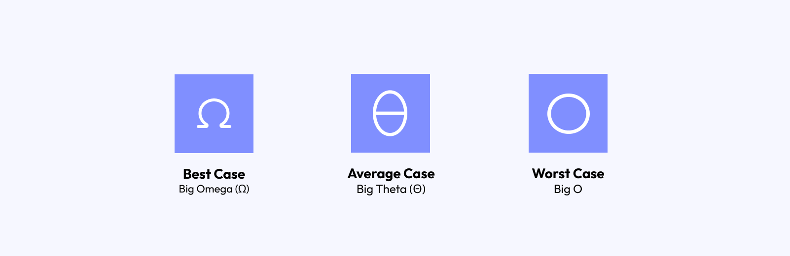
To measure how well the algorithm performs we have three types for that:

1. Best Case
2. Average Case
3. Worst Case

in most cases, we care about the worst-case scenario, like the maximum number of instructions or the maximum amount of memory that is required for a program during the running time.

There are three Greek letters associated with each of the complexity types.

let’s talk more about the Big O notation

The Big O Notation

As discussed above we use Big O for worst-case complexity, Where we want to know what are the maximum number of instructions or memory required by a program.

Below are the common time complexity using Big O notation:

O(1) - Constant Time Complexity

We use constant time complexity where the efficiency of the algorithm remains constant regardless of the input size. Any change in input size will not impact the efficiency of the program.

const compute = (input: number) => {
      return input * input * input;
}

compute(1000);

In the above example, you can see that the input size was 1000 but the number of instructions remained the same. If we make the input size 2000 it will still remain the same.

O(n) - Linear Time Complexity

We use linear complexity where the efficiency of the algorithm remains linear to the input size, Means the efficiency increase and decrease linearly based on the input size.

const compute = (input: number) => {
      let result = 0;

      for(let i = 1; i <= input; i++) {
          result += i;
      }
}

compute(10);

In the above example, you can see that the loop will run input times. if we increase or decrease the input size the efficiency will also follow it linearly.

O(n²) - Quadratic Time Complexity

We use quadratic time complexity where the efficiency of the algorithm increases quadratically to the input size. This is an indication of a nested loop which also takes n time for each of the outer n times.

const compute = (input: number) => {
      let result = 0;

      for(let i = 1; i <= input; i++) {
          for(let j = 1; j <= input; j++) {
             result += i + j;
          }
      }
}

compute(10);

in the above example, you can see that the outer loop runs from i = 1 to i = input and the inner loop runs for input times for each iteration of i, Which is a quadratic growth in complexity.

Examples of algorithms use O(n²):

1. Quick Sort
2. Bubble Sort

O(log n) - Logarithmic Time Complexity

We use logarithmic time complexity where the complexity of the algorithm increases/decreases logarithmically to the input size.

The simplest example of this can be a binary search. Where we divide the search area by half with each iteration.

Examples of algorithms use O(log n):

1. Binary Search
2. Euclidean algorithm - used to find the GCD of two numbers

O(n log n) - Log-Linear Time Complexity

We use log-linear time complexity where the complexity of the algorithm grows proportionally to n(linear complexity) multiplied by log n.

This is commonly found in algorithms where we divide the problem into subproblems (log n) and solve each of them independently (n).

Breakdown:

• n: Represents linear part where every element in input is processed at least once.
• log n: Represents logarithmic part where we divide it into sub-parts, often halving the data set.

Examples of algorithms use O(n log n):

1. Merge Sort
2. Heap Sort

That’s all for this post…